Logical Data Modeling (Part 6)

This is the sixth article in a series on logic-based approaches to data modeling. The first article[5] briefly overviewed deductive databases and illustrated how simple data models with asserted and derived facts may be declared and queried in LogiQL,[2], [13], [15] a leading-edge deductive database language based on extended datalog.[1] The second article[6]discussed how to declare inverse predicates, simple mandatory role constraints, and internal uniqueness constraints on binary fact types in LogiQL. The third article[7] explained how to declare n-ary predicates and apply simple mandatory role constraints and internal uniqueness constraints to them. The fourth article[8] discussed how to declare external uniqueness constraints in LogiQL. The fifth article[9] covered derivation rules in a little more detail and showed how to declare inclusive-or constraints.
The current article discusses how to declare simple set-comparison constraints (i.e., subset, exclusion, and equality constraints), and how to declare exclusive-or constraints. The LogiQL code examples are implemented using the free, cloud-based REPL (Read-Eval-Print-Loop) tool for LogiQL that is accessible at https://developer.logicblox.com/playground/.
Simple Subset and Exclusion Constraints, and Exclusive-Or Constraints
Table 1. Basic data about hospital patients.
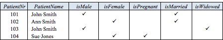
Table 1 shows an extract of a report containing basic data about hospital patients. Patients are identified by their patient number and must have their name (not necessarily unique) recorded. For each of the other five properties (e.g., isMale), a check mark "✓" indicates that the property applies to the patient, and the absence of a check mark means the property does not apply. As an optional exercise, you might like to specify a data model for this example, including all relevant constraints, before reading on.
Figure 1 models this example with a populated Object-Role Modeling (ORM)[10],[11],[12] diagram. The sample facts are shown in fact tables next to the relevant fact types. The preferred reference scheme for Patient is depicted by the popular reference mode "Nr" shown in parentheses. The uniqueness constraint bar over Patient's role in the binary fact type Patient has PatientName indicates that the relationship is many-to-one, and the mandatory role dot on the role link indicates that the role is mandatory for Patient. The NORMA tool[4] verbalizes the constraint pattern for the binary fact type as follows:
Each Patient has exactly one PatientName.
It is possible that more than one Patient has the same PatientName.
Each of the other fact types (Patient is male, etc.) is unary (only one role) and ORM fact type populations are always sets (hence no duplicates), so a uniqueness constraint is implied. The absence of a simple mandatory role constraint on the roles of the five unary fact types indicates that each of these roles is optional.
The "⊗" symbol (circled ×) connected to the "is married" and "is widowed" predicates depicts a simple exclusion constraint, indicating that for each state of the database the populations of these roles are mutually exclusive.
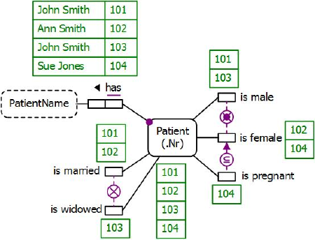
Figure 1. Populated data model for Table 1 in ORM notation.
The NORMA tool verbalizes the exclusion constraint between the "is married" and "is widowed" predicates as follows:
For each Patient, at most one of the following holds:
that Patient is married;
that Patient is widowed.
The lifebuoy symbol connected to the "is male" and "is female" predicates superimposes an inclusive-or constraint symbol "⊙" (circled mandatory role dot) with an exclusion constraint symbol "⊗" so depicts an exclusive-or constraint, indicating that each recorded patient must play at least one of these roles but not both. The NORMA tool verbalizes this constraint as follows:
For each Patient, exactly one of the following holds:
that Patient is male;
that Patient is female.
Given any two sets A and B, we say that A ⊆ B (i.e., A is a subset of B) if and only if each member of A is also a member of B. The circled subsethood operator "⊆" connected via an arrow directed from the "is pregnant" predicate to the "is female" predicate depicts a simple subset constraint, indicating that the population of pregnant patients is always a subset of the population of female patients. The NORMA tool verbalizes this subset constraint as follows:
If some Patient is pregnant then that Patient is female.
There is also an exclusion constraint between the "is male" and "is pregnant" predicates, but there is no need to assert this constraint as it is implied by the combination of the subset constraint and the exclusion component of the exclusive-or constraint.
Figure 2(a) shows the ORM schema (structure minus population) for this example. The example is also schematized in Figure 2(b) as an Entity Relationship diagram in Barker notation (Barker ER)[3], in Figure 3(c) as a class diagram in the Unified Modeling Language (UML)[16], and in Figure 2(d) as a relational database (RDB) schema.
The Barker ER schema in Figure 2(b) depicts the primary reference scheme for Patient by prepending an octothorpe "#" to the patient nr attribute. The asterisk "*" prepended to the patient nr and patient name attributes indicates that these attributes are mandatory. The small "o" prepended to the other attributes indicates that these attributes are optional.
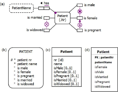
Figure 2. Data schema for Table 1 in (a) ORM, (b) Barker ER, (c) UML, and (d) relational database notation.
The UML class diagram in Figure 2(c) depicts the primary identification for Patient by appending "{id}" to the nr attribute. The nr and name attributes by default have a multiplicity of 1 so are mandatory and single-valued. The [0..1] multiplicity constraints shown on the other attributes (each of which is of type Boolean) indicates that these are optional (and have a maximum multiplicity of 1).
Figure 2(d) shows the relational database schema diagram generated by the NORMA tool[4] from the ORM schema. Here, prepending "PK" to the patientNr attribute indicates that this is the primary key of the table and hence mandatory and unique. The patientNr and patientName attributes are displayed in bold type, indicating they are mandatory (not null). The other attributes are not bolded so are optional.
The graphical notation for the Barker ER schema, the UML class diagram, and the relational database diagram cannot capture the exclusion, exclusive-or, and subset constraints depicted in the ORM schema shown in Figure 2(a). However, these constraints can be specified textually in UML using the Object Constraint Language (OCL)[17] and coded for the relational database schema using SQL check clauses.
The Figure 2(a) ORM schema may be coded in LogiQL as shown below. The right arrow symbol "->" stands for the material implication operator "→" of logic and is read as "implies". Recall that LogiQL is case-sensitive, and each formula must end with a period. The first line declares Patient as an entity type whose instances may be referenced by patient numbers that are coded as integers. The colon ":" in hasPatientNr(p:pn) distinguishes hasPatientNr as a refmode predicate so this predicate is injective (mandatory, 1:1).
The second line declares the typing constraints on the patientNameOf predicate and uses the square bracket notation to declare that the predicate is functional (many to one). The next five lines declare the typing constraints on the unary predicates. Comments are prepended by "//" and indicate the constraint declared in the code immediately following the comment. Recall that LogiQL uses an exclamation mark "!" for the not- operator (~), a comma "," for the and-operator (&), and a semicolon ";" for the inclusive-or operator (∨). The variable p in each constraint is implicitly universally quantified.
Hence the exclusion constraint coded in LogiQL as "isMarried(p) -> !isWidowed(p)." is equivalent to the logical formula "∀p[isMarried(p) → ~isWidowed(p)]". The exclusive-or constraint is coded as a combination of an inclusive-or constraint and an exclusion constraint. The inclusive-or constraint "Patient(p) -> isMale(p) ; isFemale(p)." is equivalent to the logical formula "∀p[Patient(p) → (isMale(p) ∨ isFemale(p))]", and the exclusion constraint "isMale(p) -> !isFemale(p)." is equivalent to the logical formula "∀p[isMale(p) → ~isFemale(p)]". The subset constraint coded as "isPregnant(p) -> isFemale(p)." is equivalent to the logical formula "∀p[isPregnant(p) → isFemale(p)]".
Patient(p), hasPatientNr(p:n) -> int(n).
patientNameOf[p] = pn -> Patient(p), string(pn).
isMale(p) -> Patient(p).
isFemale(p) -> Patient(p).
isPregnant(p) -> Patient(p).
isMarried(p) -> Patient(p).
isWidowed(p) -> Patient(p).// No patient is both married and widowed (e.g., could be single)
isMarried(p) -> !isWidowed(p).// Each patient is male or female but not both
Patient(p) -> isMale(p) ; isFemale(p).
isMale(p) -> !isFemale(p).// Each patient who is pregnant is female
isPregnant(p) -> isFemale(p).
To enter the schema in the free, cloud-based REPL tool use a supported browser such as Chrome, Firefox, or Internet Explorer to access the website https://repl.logicblox.com. Alternatively, you can access https://developer.logicblox.com/playground/ then click the "Open in new window" link to show a full screen for entering the code.
Schema code is entered in one or more blocks of one or more lines of code, using the addblock command to enter each block. After the "/>" prompt, type the letter "a" and click the addblock option that then appears. This causes the addblock command (followed by a space) to be added to the code window. Typing a single quote after the addblock command causes a pair of single quotes to be appended, with your cursor placed inside those quotes ready for your block of code (see Figure 3).
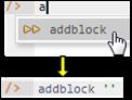
Figure 3. Invoking the addblock command in the REPL tool.
Now copy the schema code provided above to the clipboard (e.g., using Ctrl+C), then paste it between the quotes (e.g., using Ctrl+V), and then press the Enter key. You are now notified that the block was successfully added, and a new prompt awaits your next command (see Figure 4). By default, the REPL tool also appends an automatically-generated identifier for the code block. Alternatively, you can enter each line of code directly, using a separate addblock command for each line.
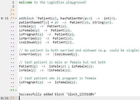
Figure 4. Adding a block of schema code.
The data in Table 1 may be entered in LogiQL using the following delta rules. A delta rule of the form +fact inserts that fact. Recall that plain, double quotes (i.e., ") are needed here, not single quotes or smart double quotes. Hence it's best to use a basic text editor such as WordPad or NotePad to enter code that will later be copied into a LogiQL tool.
+Patient(p), +hasPatientNr(p:101), +patientNameOf[p] = "John Smith", +isMale(p), +isMarried(p).
+Patient(p), +hasPatientNr(p:102), +patientNameOf[p] = "Ann Smith", +isFemale(p), +isMarried(p).
+Patient(p), +hasPatientNr(p:103), +patientNameOf[p] = "John Smith", +isMale(p), +isWidowed(p).
+Patient(p), +hasPatientNr(p:104), +patientNameOf[p] = "Sue Jones", +isFemale(p), +isPregnant(p).
Note that, unlike earlier releases, LogiQL now requires the existence of entities and their reference schemes to be explicitly declared. For example, "+Patient(p), +hasPatientNr(p:101)" is now needed to assert that there is a patient who has patient number 101, and the variable p references that patient in other facts (similarly for the other patients). A future release will allow you to omit "+Patient(p)" as the compiler will infer that from the typing constraint on a related fact assertion (e.g., +hasPatientNr(p:101)).
Delta rules to add or modify data are entered using the exec (for 'execute') command rather than the addblock command. To invoke the exec command in the REPL tool, type "e" and then select exec from the drop-down list. A space character is automatically appended. Typing a single quote after the exec command and space causes a pair of single quotes to be appended, with your cursor placed inside those quotes ready for your delta rules. Now copy the lines of data code provided above to the clipboard (e.g., using Ctrl+C), then paste it between the quotes (e.g., using Ctrl+V), and then press the Enter key. A new prompt awaits your next command (see Figure 5).

Figure 5. Adding the data below the program code.

Now that the data model (schema plus data) is stored, you can use the print command to inspect the contents of any predicate. For example, to list all the recorded patients, type "p" then select print from the drop-down list, and then type a space followed by "P", then select Patient from the drop-down list, and press Enter. Alternatively, type "print Patient" yourself and press Enter. Figure 6 shows the result. By default, the REPL tool prepends a column listing automatically-generated internal identifiers for the returned entities. Similarly, you can use the print command to print the extension of the hasPatientName, isMale, isFemale, isPregnant, isMarried, and isWidowed predicates.
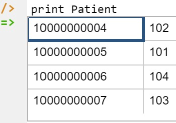
Figure 6. Using the print command to list the extension of a predicate.
As discussed in previous articles, to perform a query you specify a derivation rule to compute the facts requested by the query. For example, the following query may be used to list the patient number and patient name of each female patient. The rule's head _(pnr, pname) uses an anonymous predicate to capture the result derived from the rule's body. The variables pn and pname are head variables so are implicitly universally quantified. The variable p that is introduced in rule body is implicitly existentially quantified.
_(pnr, pname) <- hasPatientNr(p:pnr), patientNameOf[p] = pname, isFemale(p).
In LogiQL, queries are executed by appending their code in single quotes to the query command. To do this in the REPL tool, type "q", choose "query" from the drop-down list, type a single quote, then copy and paste the above LogiQL query code between the quotes, and press Enter. The relevant query result is now displayed as shown in Figure 7.

Figure 7. Using a query to list the patient number and name of the female patients.
Simple Equality Constraints
Now let's expand our model by including the latest blood pressure readings (if known) for the patients, as indicated in Table 2. Here "?" denotes a simple null, indicating unknown. Each blood pressure reading is composed of two entries, one for the systolic pressure (e.g., 120 mmHg) when the heart is at maximum contraction and one for the diastolic pressure (e.g., 80 mmHg) when the heart is fully resting.
Table 2. Blood pressure readings for patients.
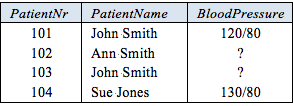
Figure 9 models this additional table as a populated ORM schema. The circled equality operator "=" connected to Patient's roles in the two blood pressure fact types depicts an equality constraint, indicating that the populations of those two roles must be equal. So each patient either has both systolic and diastolic readings taken, or neither reading. The NORMA tool verbalizes the equality constraint as follows:
For each Patient,
that Patient has some systolic BloodPressure
if and only if that Patient has some diastolic BloodPressure.
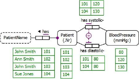
Figure 8. Populated ORM model for Table 2.
Subset, equality, and exclusion constraints are known as set-comparison constraints because they place restrictions on the comparison relationship that must apply between sets populating the relevant roles (or role sequences — which will be covered in the next article).
Figure 9(a) shows the full ORM schema for the expanded example. Figure 9(b), (c), and (d) show the expanded schema in the graphical notation of Barker ER, UML, and NORMA's relational view, none of which can display the equality constraint. However, the equality constraint can be specified textually in UML using OCL and coded for the relational database schema using an SQL check clause.
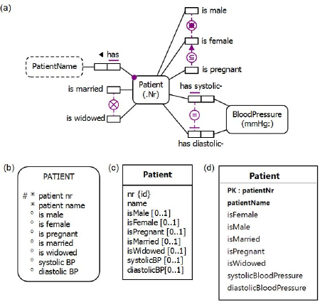
Figure 9. Expanded data model in (a) ORM, (b) Barker ER, (c) UML, and (d) relational database notation.
The additional aspects of the expanded schema may be coded in LogiQL as follows. For simplicity, blood pressure readings are modeled simply as integers. Alternatively, they could be modeled as entities using 'BloodPressure(p), has_mmHgValue(p:n) -> int(n)'. The first two lines declare the types of the two blood pressure predicates as well as their functionality. The equality constraint is declared as two subset constraints, one in each direction, using an underscore "_" for each anonymous variable (and hence existential quantification). For example, the code "systolicBPof[p] = _ -> diastolicBPof[p] = _." says that if a patient has some systolicBP then that patient also has a diastolic BP. This is equivalent to the logical formula ∀p[∃sp(p hasSystolicBP sp) → ∃dp(p hasDiastolicBP dp)].
systolicBPof[p] = sp -> Patient(p), int(sp).
diastolicBPof[p] = dp -> Patient(p), int(dp).
// For each patient, systolic bp is recorded iff diastolic bp is
systolicBPof[p] = _ -> diastolicBPof[p] = _.
diastolicBPof[p] = _ -> systolicBPof[p] = _.
Use the addblock command to add this code to the workspace in the usual way, as shown in Figure 10.
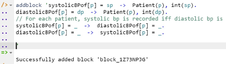
Figure 10. Adding the extra block of code to the workspace.
The additional blood pressure data may be coded in LogiQL using the following delta rules.
+Patient(p), +hasPatientNr(p:101), +systolicBPof[p] = 120, +diastolicBPof[p] = 80.
+Patient(p), +hasPatientNr(p:104), +systolicBPof[p] = 130, +diastolicBPof[p] = 80.
Now use the exec command in the usual way to enter the delta rules (see Figure 11).

Figure 11. Adding the blood pressure data to the workspace.
The following query may now be used to list the patient number, name, and blood pressure values for those patients whose latest blood pressure reading is known.
_(pnr, pname, sp, dp) <- hasPatientNr(p:pnr), patientNameOf[p] = pname, systolicBPof[p] = sp, diastolicBPof[p] = dp.
Entering this query causes the relevant result to be displayed as shown in Figure 12.

Figure 12. Querying the expanded workspace to list the known blood pressure readings.
Conclusion
The current article discussed how to declare simple subset, exclusion, and equality constraints, as well as exclusive-or constraints in LogiQL. As discussed in the next article, subset, exclusion, and equality constraints may also be declared between compound role sequences so long as these role sequences are compatible. Future articles in this series will examine how LogiQL can be used to specify business constraints and rules of a more advanced nature. The core reference manual for LogiQL is accessible at https://developer.logicblox.com/content/docs4/core-reference/. An introductory tutorial for LogiQL and the REPL tool is available at https://developer.logicblox.com/content/docs4/tutorial/repl/section/split.html. Further coverage of LogiQL may be found in [13].
References
[1] S. Abiteboul, R. Hull, & V. Vianu, Foundations of Databases, Addison-Wesley, Reading, MA (1995). ![]()
[2] M. Aref, B. Cate, T. Green, B. Kimefeld, D. Olteanu, E. Pasalic, T. Veldhuizen, & G. Washburn, "Design and Implementation of the LogicBlox System," Proc. 2015 ACM SIGMOD International Conference on Management of Data, ACM, New York (2015). http://dx.doi.org/10.1145/2723372.2742796 ![]()
[3] R. Barker, CASE*Method: Entity Relationship Modelling, Addison-Wesley: Wokingham, England (1990). ![]()
[4] M. Curland & T. Halpin, "The NORMA Software Tool for ORM 2," P. Soffer & E. Proper (Eds.): CAiSE Forum 2010, LNBIP 72, Springer-Verlag Berlin Heidelberg (2010), pp. 190-204. ![]()
[5] T.A. Halpin, "Logical Data Modeling (Part
1)," Business Rules Journal, Vol. 15, No. 5 (May 2014), URL: http://www.BRCommunity.com/a2014/b760.html ![]()
[6] T.A. Halpin, "Logical Data Modeling (Part
2)," Business Rules Journal, Vol. 15, No. 10 (Oct. 2014), URL: http://www.BRCommunity.com/a2014/b780.html ![]()
[7] T.A. Halpin, "Logical Data Modeling (Part
3)," Business Rules Journal, Vol. 16, No. 1 (Jan. 2015), URL: http://www.BRCommunity.com/a2015/b795.html ![]()
[8] T.A. Halpin, "Logical Data Modeling (Part
4)," Business Rules Journal, Vol. 16, No. 7 (July 2015), URL: http://www.BRCommunity.com/a2015/b820.html ![]()
[9] T.A. Halpin, "Logical Data Modeling (Part
5)," Business Rules Journal, Vol. 16, No. 10 (Oct. 2015), URL: http://www.BRCommunity.com/a2015/b832.html ![]()
[10] T.A. Halpin, Object-Role Modeling Fundamentals, Technics Publications: New Jersey (2015). ![]()
[11] T.A. Halpin, Object-Role Modeling Workbook, Technics Publications: New Jersey (2016). ![]()
[12] T.A. Halpin & T. Morgan, Information Modeling and Relational Databases, 2nd edition, Morgan Kaufmann: San Francisco (2008). ![]()
[13] T.A. Halpin & S. Rugaber, LogiQL: A Query language for Smart Databases, CRC Press: Boca Raton (2014); http://www.crcpress.com/product/isbn/9781482244939# ![]()
[14] T.A. Halpin & J. Wijbenga, "FORML 2," Enterprise, Business-Process and Information Systems Modeling, eds. I. Bider et al., LNBIP 50, Springer-Verlag, Berlin Heidelberg (2010), pp. 247–260.
[15] S. Huang, T. Green, & B. Loo, "Datalog and emerging applications: an interactive tutorial," Proc. 2011 ACM SIGMOD International Conference on Management of Data, ACM, New York (2011). At: http://dl.acm.org/citation.cfm?id=1989456 ![]()
[16] Object Management Group, OMG Unified Modeling Language Specification (OMG UML), version 2.5 RTF Beta 2, Object Management Group (2013). Available online at: http://www.omg.org/spec/UML/2.5/ ![]()
[17] Object Management Group, OMG Object Constraint Language (OCL), version 2.3.1, Object Management Group (2012). Retrieved from http://www.omg.org/spec/OCL/2.3.1/ ![]()
# # #
Standard citation for this article:
About our Contributor:

")


Online Interactive Training Series
In response to a great many requests, Business Rule Solutions now offers at-a-distance learning options. No travel, no backlogs, no hassles. Same great instructors, but with schedules, content and pricing designed to meet the special needs of busy professionals.
How to Define Business Terms in Plain English: A Primer
How to Use DecisionSpeak™ and Question Charts (Q-Charts™)
Decision Tables - A Primer: How to Use TableSpeak™
Tabulation of Lists in RuleSpeak®: A Primer - Using "The Following" Clause
Business Agility Manifesto
Business Rules Manifesto
Business Motivation Model
Decision Vocabulary
[Download]
[Download]
Semantics of Business Vocabulary and Business Rules